DSA 250: Housing Price Analysis
By: Delilah Hollander | Course: DSA 250 — Data Science & Analytics
1. Project Overview
For DSA 250, I analyzed 1,460 home sales in Ames, Iowa to identify which home features most strongly predict sale price. I examined four predictors — square footage, bathrooms, year built, and bedrooms — first with exploratory analysis, then built a multiple linear regression model to quantify each variable's true impact and make predictions.
Research Questions:
- How strongly does above-ground square footage predict sale price?
- Do homes with more full bathrooms sell for more?
- Are newer homes priced higher than older ones?
- Does bedroom count still predict price once size is controlled for?
2. Data Source & Preparation
Source: Ames Housing Dataset (Kaggle — 81 original columns, 1,460 rows). I narrowed it to 5 key variables.
# Select key variables and drop any incomplete rows
key_vars = ['SalePrice', 'GrLivArea', 'BedroomAbvGr', 'FullBath', 'YearBuilt']
df_clean = df[key_vars].dropna()
# Result: 0 rows dropped — all 1,460 records were complete
A .isnull().sum() check confirmed zero missing values in all five variables — no imputation needed.
3. Exploratory Data Analysis
Distributions
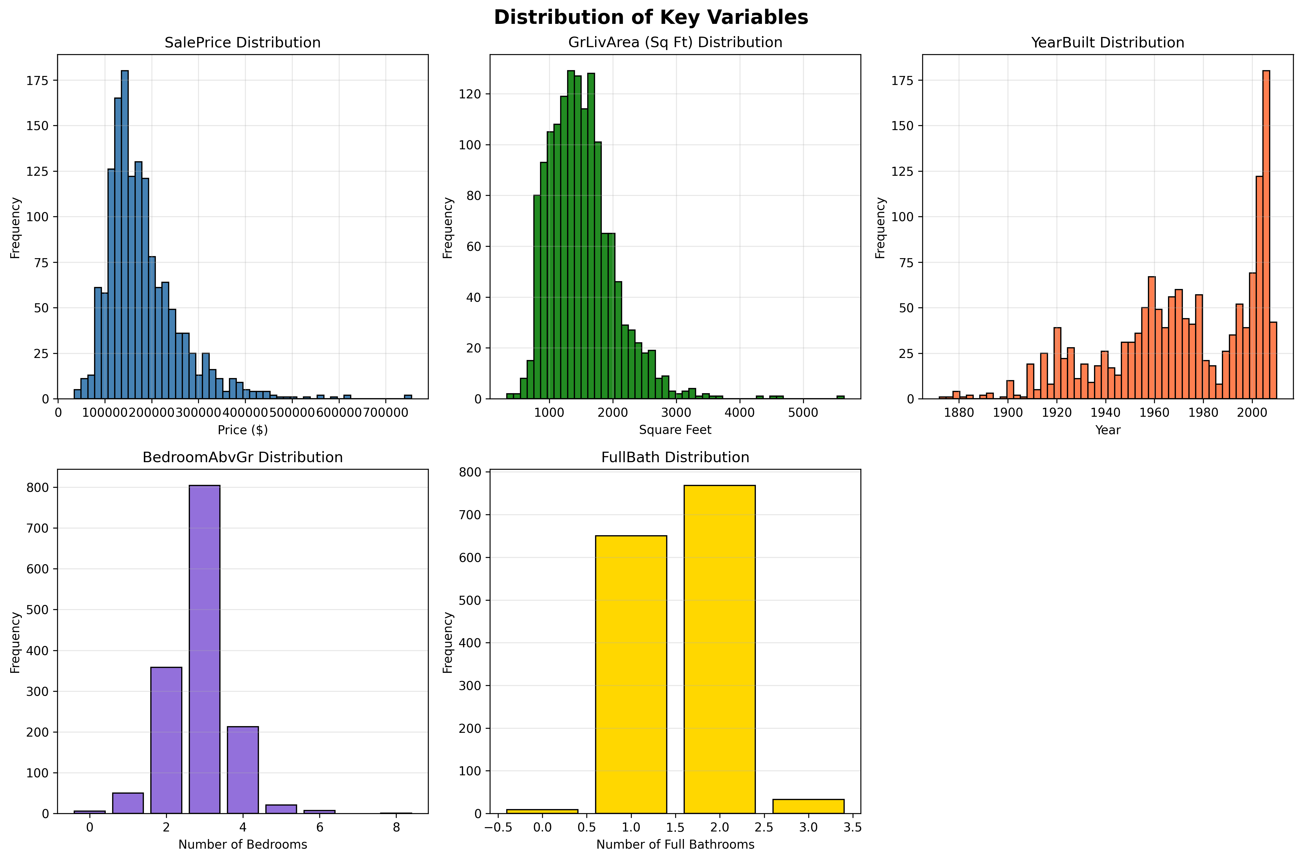
SalePrice and GrLivArea are both right-skewed — most homes are moderate in size and price, but a few large, expensive properties pull the average up. Bedroom and bathroom counts are more symmetric and discrete.
Correlation Heatmap
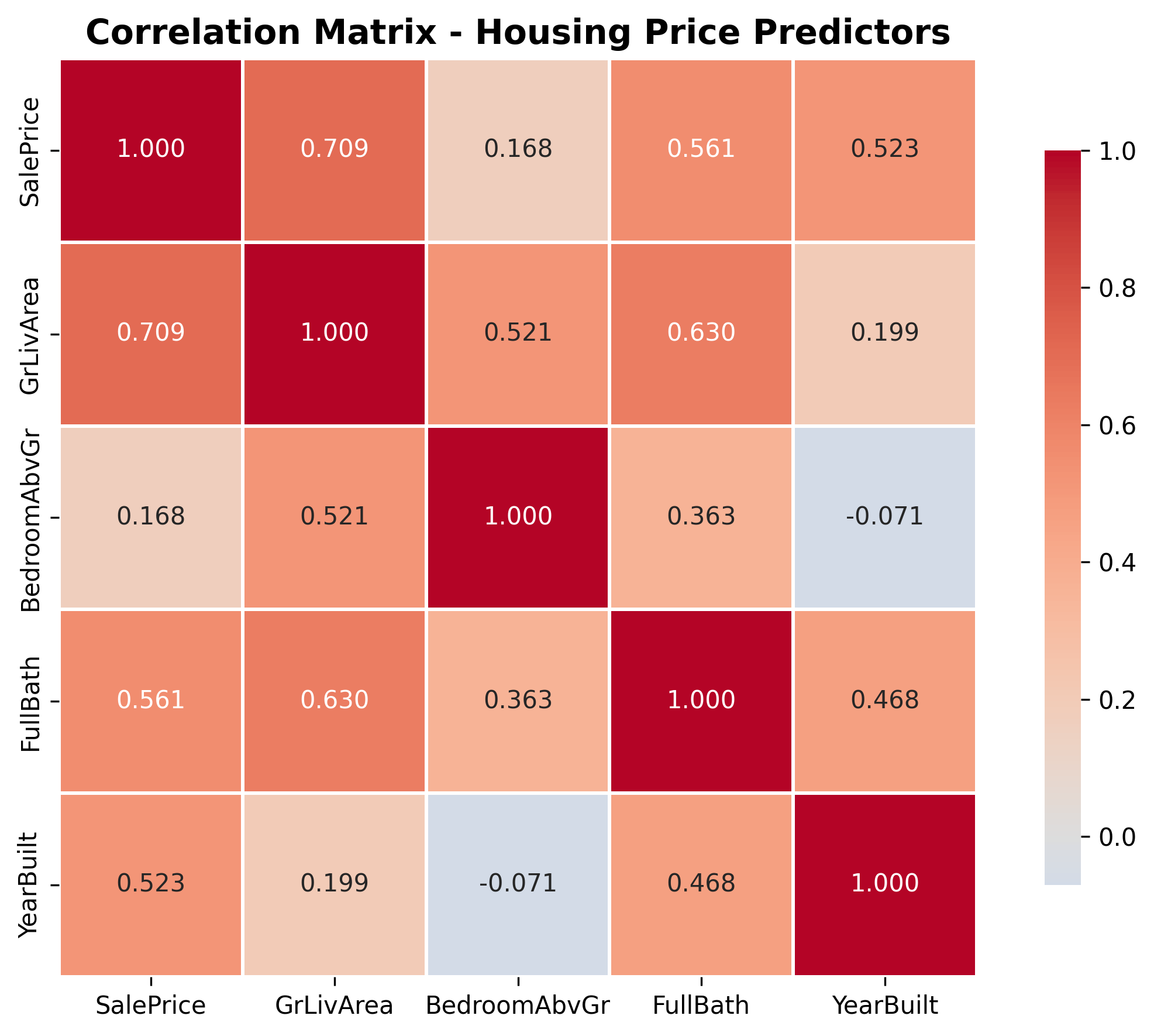
The heatmap shows that GrLivArea (r = 0.709) and FullBath (r = 0.561) are the strongest individual predictors of SalePrice. Bedroom count (r = 0.168) is surprisingly weak — likely because bigger homes tend to have more bedrooms, so square footage accounts for most of that signal.
4. Color-Encoded Scatter Plots
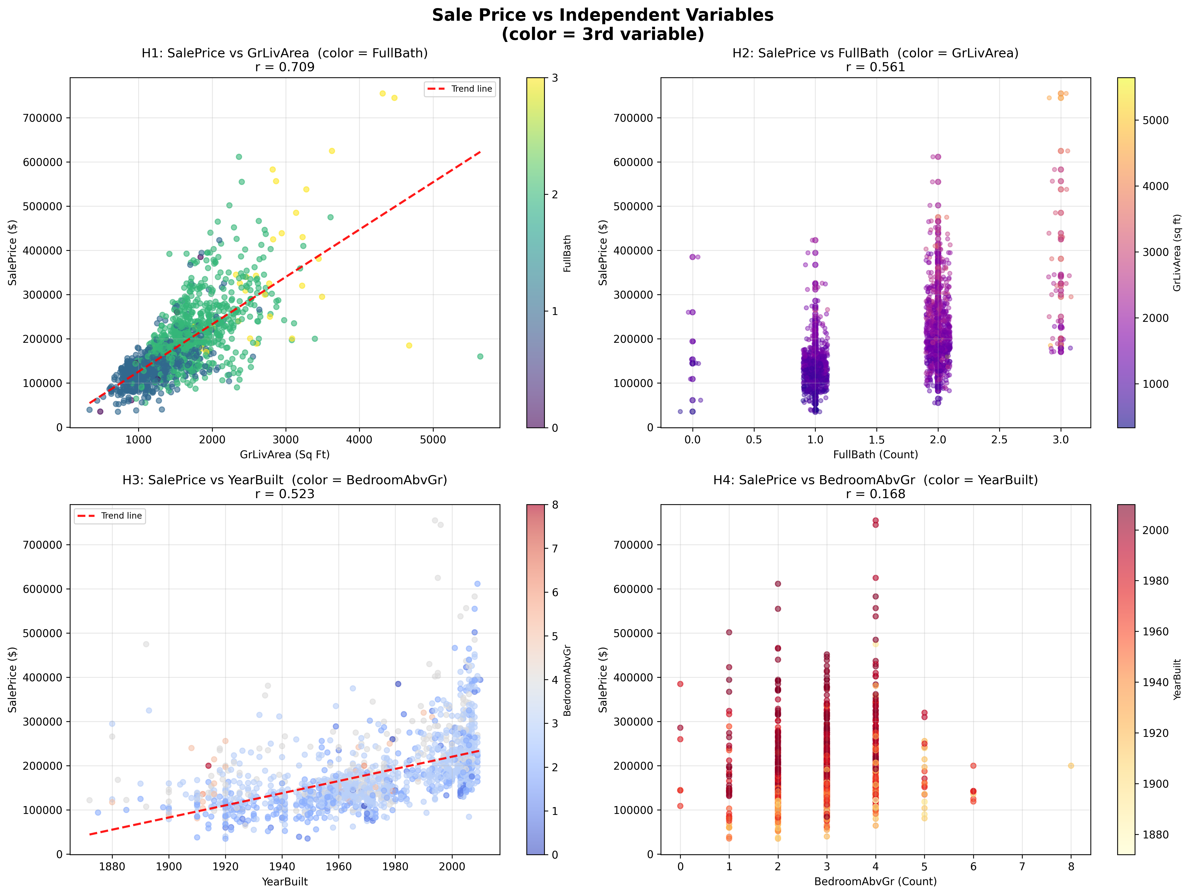
Each scatter plot uses color to encode a third variable, revealing multi-dimensional relationships at a glance:
- Top-left (LivArea vs Price, color = FullBath): Larger homes tend to have more baths AND cost more — all three rise together.
- Top-right (FullBath vs Price, color = GrLivArea): High-bath, high-price homes are also the largest.
- Bottom-left (YearBuilt vs Price, color = Bedrooms): Newer homes command higher prices regardless of bedroom count.
- Bottom-right (Bedrooms vs Price, color = YearBuilt): 3-bedroom homes are most common; newer ones fetch notably higher prices.
5. Linear Regression Model
I fit two models using scikit-learn, training on 80% of the data (1,168 homes) and testing on the remaining 20% (292 homes).
Simple Regression
GrLivArea → SalePrice only
| RMSE | $58,472 |
| MAE | $38,341 |
| Slope | $102.49 / sq ft |
Multiple Regression
All 4 features → SalePrice
| RMSE | $47,468 |
| MAE | $32,045 |
| Improvement | +15.2 pp over simple |
Model Equation
+ $107.17 × GrLivArea
− $16,947 × BedroomAbvGr
− $1,588 × FullBath (controlled for size)
+ $960 × YearBuilt
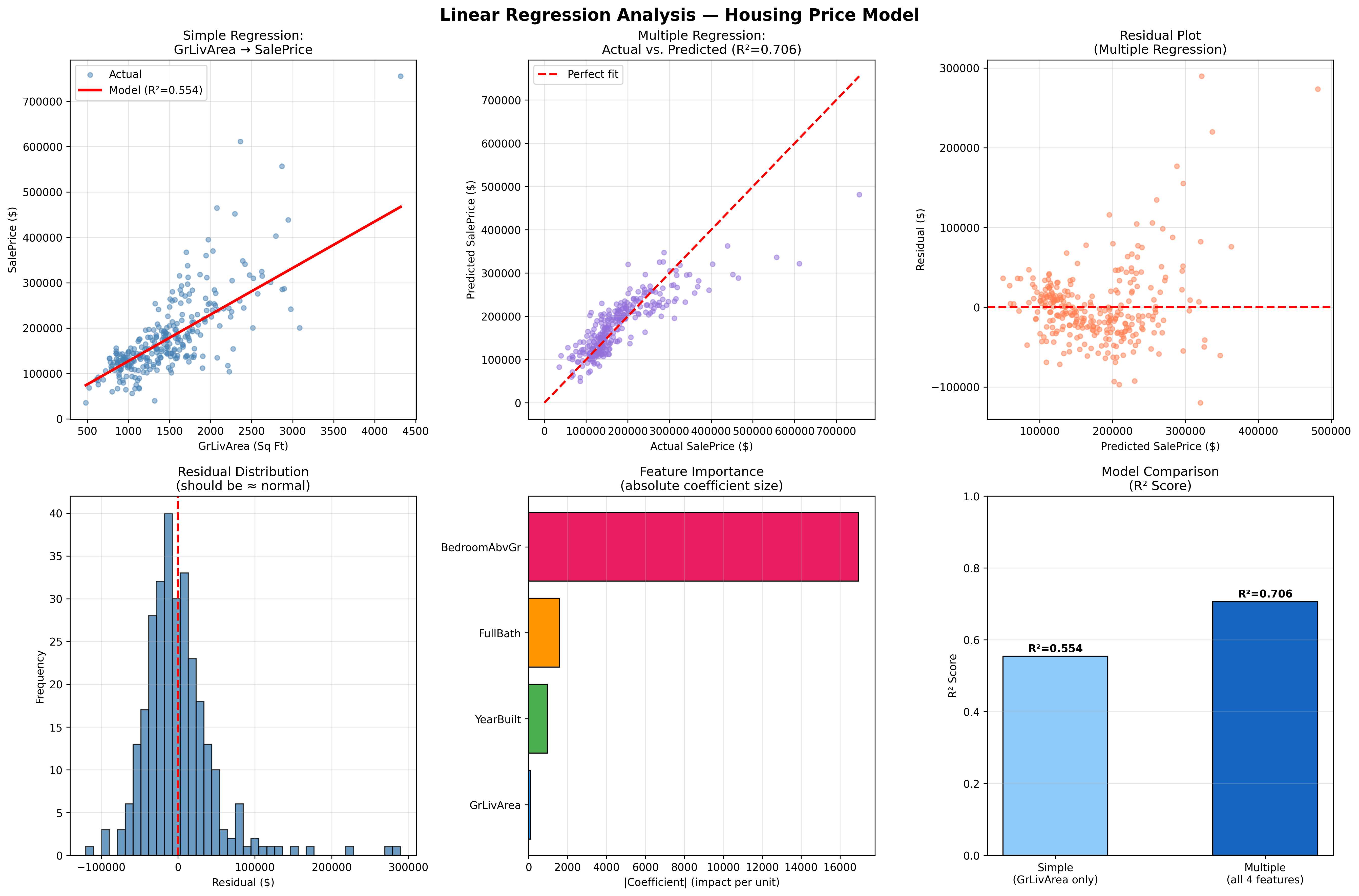
Why is the bedroom coefficient negative? Once square footage is in the model, adding more bedrooms to the same square footage means smaller rooms — which buyers actually value less. This is a classic example of multicollinearity.
Regression Diagnostics
The diagnostic panel includes: simple vs multiple regression lines, predicted vs actual plot, residual plot, residual distribution, feature importance, and model comparison.
6. Sample Predictions
These predictions were generated by the trained multiple regression model (not a hand-coded formula). The ±1σ range uses the model's RMSE of $47,468.
| Sq Ft | Beds | Baths | Year Built | Predicted Price | Likely Range |
|---|---|---|---|---|---|
| 1,000 | 2 | 1 | 1960 | $130,399 | $82,931 – $177,867 |
| 1,500 | 3 | 1 | 1990 | $195,837 | $148,369 – $243,305 |
| 2,000 | 3 | 2 | 2000 | $257,434 | $209,966 – $304,902 |
| 2,500 | 4 | 2 | 2005 | $298,873 | $251,405 – $346,341 |
| 3,000 | 4 | 3 | 2010 | $355,670 | $308,202 – $403,138 |
Note: ±1 RMSE uncertainty band = ±$47,468. The model explains 70.6% of price variance on held-out test data.
7. Key Takeaways
Square footage is king. GrLivArea (r = 0.709) is the dominant predictor. Each additional sq ft adds roughly $107 in sale price. It's the single most powerful variable in both the simple and multiple models.
Bathrooms are a better investment than bedrooms. FullBath (r = 0.561) has more than 3× the correlation of bedroom count (r = 0.168). If you're renovating to sell, add a bath before a bedroom.
The age gap is real money. YearBuilt (r = 0.523) contributes roughly $960 per year newer. A 1950 vs. 2005 home at the same size could differ by ~$52,000.
Multiple regression explains 70.6% of price variance — a 15.2-point R² gain over the single-variable model. Real-world limitations (neighborhood quality, remodels, lot size) explain the remaining ~30%.